Introduction
This script was inspired by a discussion on LinkedIn following up from a cross post of an article on Nightingale by Nick Desbarats. I was to reproduce the graphs using MATLAB. So lets go through this in the form of a live script, which you can directly download if you want.
Boilerplate
Force the seed on the random number generator, normally not a good practice, but great for examples here.
clearvars
close all
rng(1)
Generate Some Dummy Data
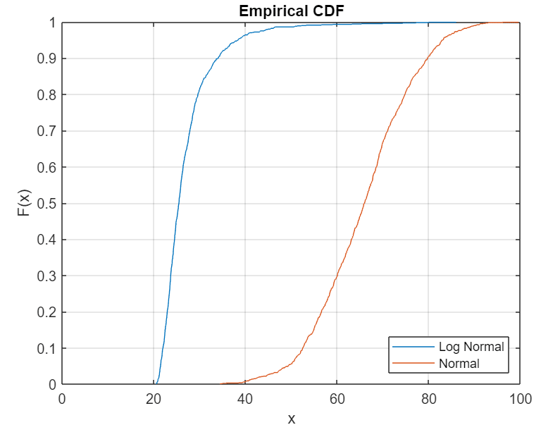
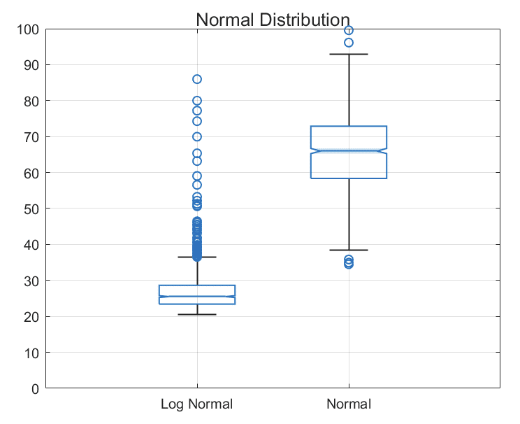
So lets just generate some dummy data from a normal distribution and a log normal distribution. Lets then visualise with a cumulative probability plot and set our baseline box plots
Data Generation
nSamples = 1000;
distLogNormal = makedist("Lognormal","mu", 1, "sigma", 0.75);
dataLN = random(distLogNormal, [nSamples, 1]);
dataLN = (dataLN + 10) * 2;
distNormal = makedist("Normal", "mu", 65, "sigma", 10);
dataN = random(distNormal, [nSamples, 1]);
Cumulative Distribution Plots
figure
cdfplot(dataLN)
hold on
cdfplot(dataN)
hold off
legend(["Log Normal", "Normal"], ...
    Location="southeast")
xlim([0 100])
Base Line Box Plots
figure
boxchart([dataLN, dataN], 'Notch','on')
xticklabels(["Log Normal", "Normal"])
ylim([0 100])
box on
grid on
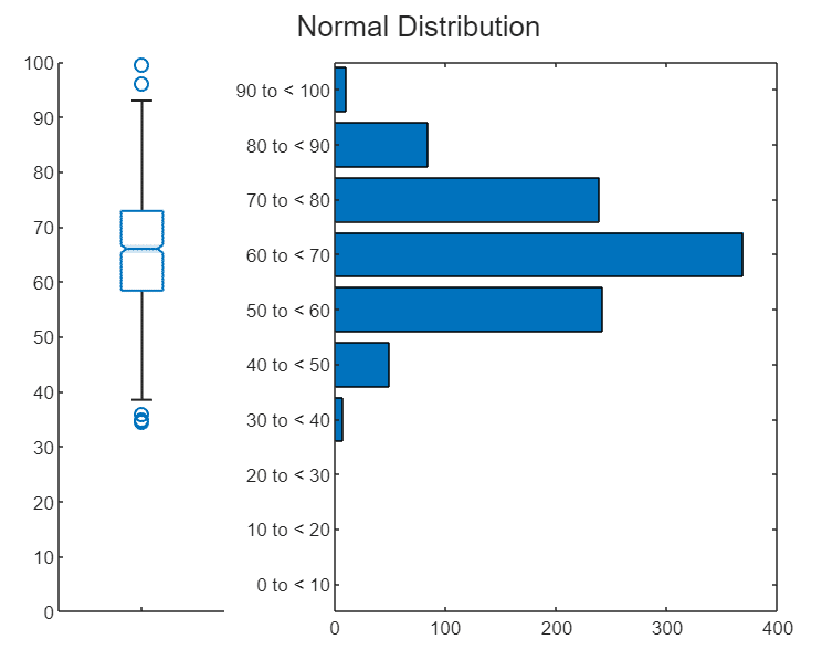
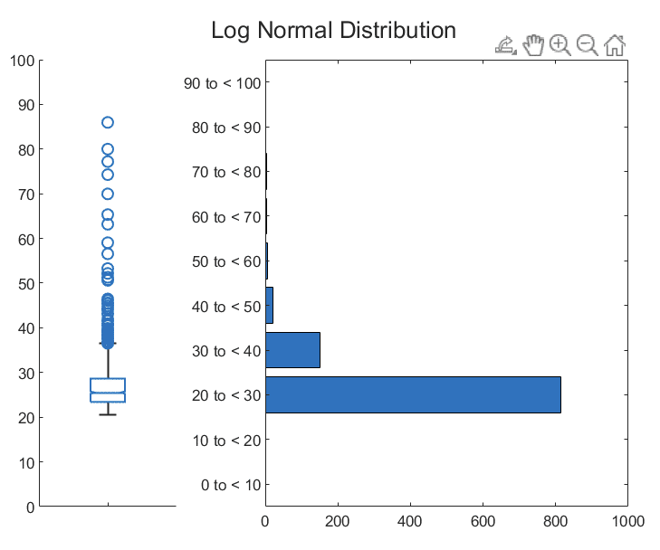
Side-By-Side Comparison Plot
Normal Distribution
figure
plotBoxBar(dataN, "Normal Distribution")
Log Normal Distribution
figure
plotBoxBar(dataLN, "Log Normal Distribution")
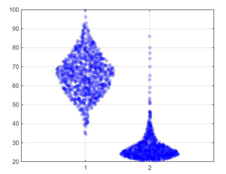
Simple Violin Plots – AKA Swarm Charts
figure
swarmchart([ones(nSamples, 1) ones(nSamples, 1)*2], [dataN, dataLN], ...
    'blue', ...
    'filled', ...
    'MarkerFaceAlpha',0.25, ...
    'MarkerEdgeAlpha',0.25, ...
    'XJitter','density')
xlim([0 3])
xticks(1:2)
box on
grid on
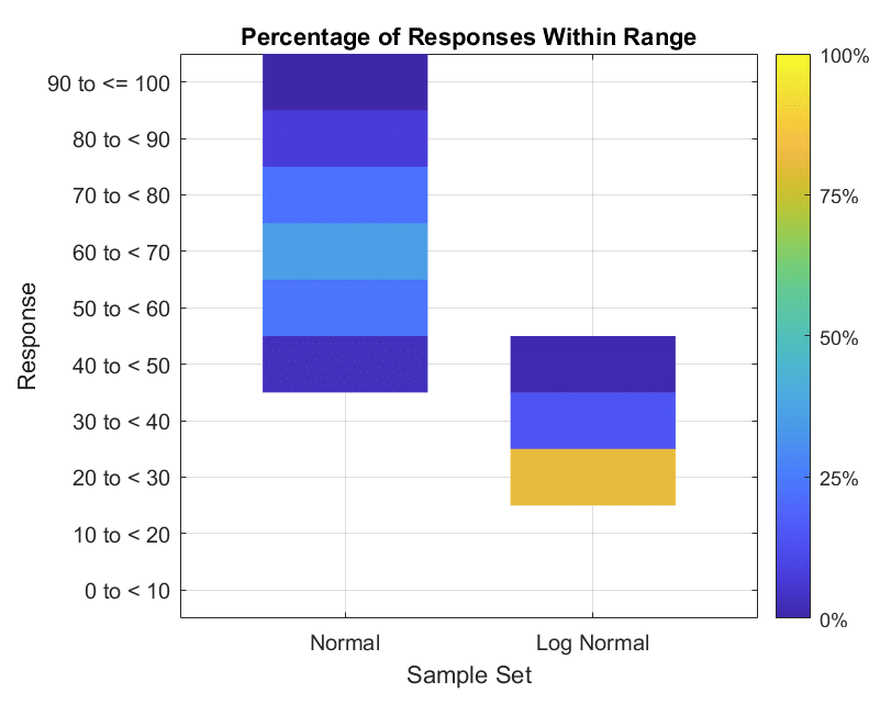
Box Bar Intensity Plots
binEdges = 0:10:100;
yN = histcounts(dataN, binEdges) / nSamples;
yLN = histcounts(dataLN, binEdges) / nSamples;
figure
c = parula(100);
basePatchX = [-0.5 0.5 0.5 -0.5];
basePatchY = [-0.5 -0.5 0.5 0.5];
for ii = 1:numel(binEdges)-1
    if floor(yN(ii) * 100) > 0
        patch(basePatchX + 1 - 0.5, ...
            basePatchY + ii, ...
            'r', ...
            'FaceColor', c(floor(yN(ii) * 100), :), ...
            'LineStyle', 'none')
    end
    if floor(yLN(ii) * 100) > 0
        patch(basePatchX + 2, ...
            basePatchY + ii, ...
            'r', ...
            'FaceColor', c(floor(yLN(ii) * 100), :), ...
            'LineStyle', 'none')
    end
end
ylim([0.5 10.5])
yticklabels([ ...
    "0 to < 10", ...
    "10 to < 20", ...
    "20 to < 30", ...
    "30 to < 40", ...
    "40 to < 50", ...
    "50 to < 60", ...
    "60 to < 70", ...
    "70 to < 80", ...
    "80 to < 90", ...
    "90 to <= 100"])
xticks([0.5 2])
xticklabels(["Normal", "Log Normal"])
xlim([-0.5 3])
colorbar('Ticks', 0:0.25:1, ...
    'TickLabels', ["0%", "25%", "50%", "75%", "100%"])
title('Percentage of Responses Within Range')
ylabel("Response")
xlabel("Sample Set")
box on
grid on
Support Functions
function plotBoxBar(data, titleText)
t = tiledlayout(1,3, ...
    TileSpacing="compact");
nexttile
boxchart(data, 'Notch','on')
xticklabels("");
ylim([0 100])
nexttile(2, [1, 2])
y = histcounts(data, 0:10:100);
barh(5:10:95, y)
ylim([0 100])
yticklabels([ ...
    "0 to < 10", ...
    "10 to < 20", ...
    "20 to < 30", ...
    "30 to < 40", ...
    "40 to < 50", ...
    "50 to < 60", ...
    "60 to < 70", ...
    "70 to < 80", ...
    "80 to < 90", ...
    "90 to < 100"])
title(t, titleText)
end